BIBLIOTHECA AUGUSTANA
Ernst Ising
1900 - 1998
Contribution to theTheory of Ferromagnetism
1925
|
|||||||||||||||
|
______________________________________________________________________________
|
|||||||||||||||
2. The simple linear chain.
We want to apply these propositions to a model as simple as possible. We calculate the middle moment J of a linear magnet consisting of n elements. Each of these n elements should be able to take only two positions in which its moment m points in the ordered direction of the chain. We distinguish the two possible directions by the designations positive and negative, in short, we speak of positive and negative elements.In order to calculate J, we consider an arrangement of the chain with ν1 positive and ν2 negative elements, such that
ν1 + ν2 = n. (1)
For s positions, there will be negative elements inserted between the positive ones, i.e. on each of these s positions there is a group of negative elements which are connected to each other. For instance, for s = 3 we have
|
|||||||||||||||


(2) |
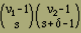
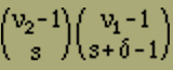
gives the number of arrangements described above. One obtains the number of corresponding arrangements beginning left with a negative element if one exchanges ν1 and ν2 in (2); it is therefore
(2') |
We establish that the inner energy disappears when all elements are similarly oriented. But if similar poles of neighboring elements (i.e. positive and negative elements as designated above) interact on (2s + δ) positions (namely the 2s borders of the gaps and the edge of the remaining group on the right end), as is the case in the above considered arrangement, then such an arrangement should have the inner energy
(2s + δ) · ε (ε > 0)
Since the moment of our arrangements is
(ν1 - ν2) m (3)
their total energy in an outer magnetic field
(2s + δ)ε + (ν2 - ν1) (mH) (3')
To abbreviate we set
(4) |
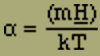
where k = 1.37 · 10-16, the Boltzmann constant, and T is the absolute temperature. To calculate the middle moment J, using equations (2), (2'), (3') and (4), we find the sum
(5) |
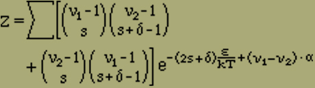
Since in deriving Z from α, each member multiplies with (ν1 - ν2), namely with the moment belonging to it (3) except for the factor m, the middle moment can be obtained in the form
(6) |
Equation (5) has to be summed up over ν1 and ν2 with the side condition (1) over s from 0 to infinity and for δ = 0.1 - for too large values of s the binomial coefficients disappear.
These summations are easy to perform if one considers the partition function Z(n) as a function of n and eliminates the side condition (1) by forming with the help of an arbitrary mathematical auxiliary variable x
(7) |
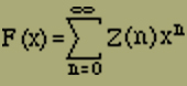
where n in Z means ν1 + ν2. The calulation of F(x) is done by summing up from 0 to infinity over ν1 and ν2 independently of each other which can be done without difficulty with the help of the binomial theorem. When this has been done, we only have a geometrical series before us whose summation gives us
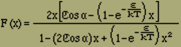
If one develops again this closed expression for F(x) by means of further continued fraction analysis for powers of x, one finds as coefficient of xn

c1 and c2 are used here for abbreviations for two factors which do not play any part in the following; c1 is for all values of magnitude 1. In Z one can neglect the factor
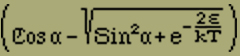
since this quantity is always < 1, while
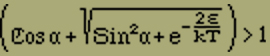
and because n is a very large number. Since one can neglect the contribution of c1 from

because n > 1, one finds, according to equation (6),
(8) |
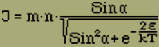
This function disappears for H = 0, i.e. α = 0; thus we find no appearances of hysteresis and no spontaneous magnetization. An increase of ε only causes a change in the form of the curve, so that saturation is reached more quickly and more completely.
Two reasons can be found for this behavior. Thus, if one considers H = 0, the probabilities as a function of the moment M, this curve has either two maxima symmetrically positioned around M = 0, and probably very steep, or, for reasons of symmetry, a single maximum at M = 0. From the result J = 0 of the average, one cannot, when the curve of the probabilities has two maxima, necessarily draw the conclusion that the middle moment, which is to be observed, disappears. It would be much more reasonable that the state of the magnet fluctuates for longer times, (compared to the length of the observation) around one of the two most probably equal moments which are opposite to each other and that thereby spontaneous magnetization could be observed. Unfortunately a simple calculation shows that the possibilities only have a simple maximum. Thus the larger expenditure of energy of the nonmagnetic state is compensated for by its extraordinarily large complexity.
As an analogous examination shows 2), nothing is changed in the result J = 0 for H = 0, when we include for the elements, besides the positive and negative positions, further orientations perpendicular thereto, or when we consider the mutual effect of second order elements next to the neighboring elements.
――――――――――